Saturday, October 11, 2008

Merging GPS logs and mapping them all

Inspired by cabspotting and Open Street Map, I wanted to merge all my GPS logs and create a map showing all the routes I've logged lately.

This is pretty easy using gpsbabel, but I needed to use a little Python to get the list of input log files. (I'm sure there's a way to do it in bash but that's beyond me for now.) My GPS stores files in nmea format, and the directory structure/purpose of my Python script should hopefully be apparent.

>>> import os
>>> from path import path
>>> logs = " ".join([" ".join(["-i nmea -f %s"%log
                               for log in sorted((raw/"raw").files("GPS_*.log"))]) 
                     for raw in path("/home/tom/docs/gpslogs").dirs() 
                     if raw.namebase.isdigit()])
>>> logs
'-i nmea -f /home/tom/docs/gpslogs/200810/raw/GPS_20080930_221152.log -i nmea -f /home/tom/docs/gpslogs/200810/raw/GPS_20081001_071234.log ...'
>>> os.system("gpsbabel %s -o kml,points=0,labels=0,trackdata=0 -F /home/tom/docs/gpslogs/all200810.kml" % logs)

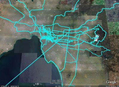
The result of that is a 36.5 MB kml file I could load into Google Earth:

There was one spurious point somewhere in the log file at 0° E, 0° N, and the log has a lot of jitter when I'm walking near home.

Thursday, September 18, 2008

A simple game using JavaScript and the CANVAS element

This should work in Opera and Firefox (though really slowly, why I don't know) and probably Safari. It's not going to work in IE because I can't be bothered getting the iecanvas thingi into the blog code.

Update: There is now an iPhone version.

The only thing to note is less clicks == better score.

Canvas not supported...
Clicks
0
0000

Monday, August 25, 2008

Analysing GPS Logs with Awk

This post describes the first two "chop" functions that fit into the partitioning framework outlined last post.

def chopToSpeedHistogram(dest, p):
    # create histogram of speeds from nmea written to stdout
    os.system("cat "+sh_escape(dest)+".log"
              + " | awk -F , '{if($1==\"$GPVTG\" && int($8)!=0){count[int($8+0.5)]++}}"
              + " END {for(w in count) printf(\"[%d,%d],\\n\", w, count[w]);}'"
              # sort it
              + " | sort -g -k 1.2"
              # output json of histogram
              + " > "+sh_escape(dest)+".hist")

def chopToHeadingHistogram(dest, p):
    # create histogram of headings from nmea written to stdout (ignore heading when stopped)
    os.system("cat "+sh_escape(dest)+".log"
              + " | awk -F , '{if($1==\"$GPVTG\" && int($8)!=0){count[5.0*int($2/5.0+0.5)]++;}}"
              + " END {for(w in count) printf(\"[%d,%d],\\n\", w, count[w]);}'"
              # sort it
              + " | sort -g -k 1.2"
              # output json of histogram
              + " > "+sh_escape(dest)+".head")

Both functions use awk to create a histogram from the speed (in km/h) and heading (or bearing, in degrees) from the NMEA VTG sentences. The speed is rounded to an integer, and the bearing to the nearest 5 degrees. The data logger records on reading per second, so this gives a measure of how much time was spent at each speed/bearing.

The histogram is output in a "json" array format that can be inserted straight into a webpage where the flot library is used to generate some graphs.

Speed Histogram

The average and standard deviation (shaded at ±0.5σ) are indicated on the graph for two bike rides along the same route, and match pretty closely with that recorded by my bike computer:

GPS logBike computer
Ride 1 (brown) 2hrs 59 min, minus 41 min stopped63.4km27.7km/h 2 hrs 16 min64.01km28.00km/h
Ride 2 (dark green) 2 hrs 25 min, minus 13 min stopped63.4km29.0km/h 2 hrs 10 min63.85km29.30km/h

The two rides went in different directions, the first in the "uphill" direction and the second with a bit of a tail wind. I got a flat tire on the first ride too, hence the extra time spent stopped.

Heading Histogram

Up is north and the radius represents the time spent heading in that direction (normalized during the plotting process and "expanded" by taking the square root to show a little more detail.)

Thursday, August 21, 2008

Automatically Partitioning GPS Logs with gpsbabel

My GPS logger is capturing lots of useful information but it's difficult to efficiently capture data for regular activities. Geotagging photos is easy, and manually working with the logs for a special event is possible, but it's not feasible to put in that much work to analyze commutes for example.

The logger creates a separate log file each time it's switched on and off, and while these logs could be sorted into categories for analysis, it's easy to forget to turn it on and off at the start and end of a section of interest and activities are then merged in the logs. In addition, there is often "junk" data at start and end of logs while leaving or arriving at a destination.

I wanted to be able to automatically capture the information about my daily activities by simply switching on the logger and carrying it around with me. I then simply want to plug the logger into the computer and have the logs automatically chopped into segments of interest that can be compared to each other over time.

The rest of this post roughly outlines the Python script I created to perform this task, minus some of the hopefully irrelevant details.

Firstly, I collect the lat/long coordinates of places that I am interested in collecting data while I'm there and traveling between them. These include my home, work, the climbing gym and so on. Each point has a radius within which any readings will be considered to be in that place.

#         id:  name lat         long        radius
places = { 1: ("A", -37.123456, 145.123456, 0.050),
           2: ("B", -37.234567, 145.234567, 0.050),
           3: ("C", -37.345678, 145.345678, 0.050) }
otherid = 4

For each of these places of interest, I then use gpsbabel's radius filter to find all the times where I was within that zone:

# create a list of all raw log files to be processed
from path import path
month = path("/gpslogs/200808")
logs = " ".join(["-i nmea -f %s"%log 
                 for log in sorted((month/"raw").files("GPS_*.log"))])

for (id,(place,lat,lon,radius)) in places.items():
   os.system("gpsbabel "
             # input files
             + logs
             # convert to waypoints
             + " -x transform,wpt=trk,del"
             # remove anything outside place of interest
             + (" -x radius,distance=%.3fK,lat=%.6f,lon=%.6f,nosort"%(radius,lat,lon))
             # convert back to tracks
             + " -x transform,trk=wpt,del"
             # output nmea to stdout
             + " -o nmea -F -"
             # filter to just GPRMC sentences
             + " | grep GPRMC"
             # output to log file
             + (" > %s/processed/place%d.log"%(month,id)))

And all points outside any of the specific places of interest are sent into an "other" file:

os.system("gpsbabel "
          # input files
          + logs
          # convert to waypoints
          + " -x transform,wpt=trk,del"
          # remove anything in a place of interest
          + "".join([" -x radius,distance=%.3fK,lat=%.6f,lon=%.6f,nosort,exclude"%(radius,lat,lon)
                     for (id,(place,lat,lon,radius)) in places.items()])
          # convert back to tracks
          + " -x transform,trk=wpt,del"
          # output nmea to stdout
          + " -o nmea -F -"
          # filter to just GPRMC sentences
          + " | grep GPRMC"
          # output to log file
          + (" > %s/processed/place%d.log" % (month, otherid)))

These files are filtered with grep to contain only minimal data as we only require the timestamps for this part of the process. Specifically only the NMEA GPRMC sentences are kept.

To provide a brief illustration, the following picture shows two log files of data, a blue and a green, between three points of interest:
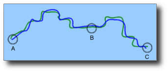
The above process would create four files, one for each point A, B and C and one for "Other" points that would contain something like the following information, where the horizontal axis represents time:

I then read all those log files back in to create a "time line" that for each timestamp stores my "location" in the sense that it knows whether I was "home", at "work" or somewhere between the two.

# dict of timestamp (seconds since epoch, UTC) to placeid
where = {}
for placeid in places.keys()+[otherid,]:
   for line in (month/"processed"/("place%d.log"%placeid)).lines():
      fields = line.split(",")
      # convert date/time to seconds since epoch (UTC)
      t, d = fields[1], fields[-3]
      ts = calendar.timegm( (2000+int(d[4:6]), int(d[2:4]), int(d[0:2]),
                             int(t[0:2]), int(t[2:4]), int(t[4:6])) )
      where[ts] = placeid

This is then summarised from one value per second to a list of "segments" with a start and end time and a location. Unlogged time segments are also inserted at this point whenever there are no logged readings for 5 minutes or more.

# array of tuples (placeid, start, end, logged)
# placeid = 0 indicates "unknown location", i.e. unlogged
summary = []
current, start, stop, last_ts = 0, 0, 0, None
for ts in sorted(where.keys()):
   # detect and insert "gaps" if space between logged timestamps is greater than 5 minutes
   if last_ts and ts-last_ts > 5*60:
      if current:
         summary.append( [current, start, stop, True] )
      current, start, stop = where[ts], ts, ts
      summary.append( [0, last_ts, ts, False] )
 
   last_ts = ts

   if where[ts] != current:
      if current:
         summary.append( [current, start, stop, True] )
      current, start, stop = where[ts], ts, ts
   else:
      stop = ts
summary.append( [current, start, stop, True] )

(If there's a more "Pythonic" way of writing that kind of code, I'd be interested in knowing it.)

"Spurious" segments are then removed. These show up because when the logger is inside buildings the location jumps around and often out of the 50m radius meaning that, for example, there will be a sequence of Home-Other-Home-Other-Home logs. The "Other" segments that are between two known points of interest and less than 5 minutes long are deleted, as are "Other" segments that sit between a known place of interest and an unlogged segment.

Based on the above graphic, the summary might look something like the following:

startendlocation
10.00am10.05amA
10.05am10.30amOther
10.30am10.35amB
10.35am11.00amOther
...

The "Other" segments are then labelled if possible to indicate they were "commutes" between known locations:

startendlocation
10.00am10.05amA
10.05am10.30amA-B
10.30am10.35amB
10.35am11.00amB-C
...

Some segments cannot be labeled automatically and are left as "Other". This may be a trip out to a "one-off" location and back again, which can be left as "Other". However, sometimes it is because the logger didn't lock onto the satellites within the 50m radius on the way out of a place of interest and these can be manually fixed up later.

Once a list of "activities" has been obtained, with start and end times, it is easy to use gpsbabel again to split logs based on start and end of time segments:

for (place, start, stop, place_from, place_to, logged) in summary:
    dest = month / "processed" / ("%s-%s"%(time.strftime("%Y%m%d%H%M%S", time.localtime(start)),
                                           time.strftime("%Y%m%d%H%M%S", time.localtime(stop))))

   for (ext, chopFn) in [(".log", chopToLog),
                         (".kml", chopToKml), 
                         (".speed", chopToSpeedVsDistance), 
                         (".alt", chopToAltitudeVsDistance), 
                         (".hist", chopToSpeedHistogram),
                         (".head", chopToHeadingHistogram),
                         (".stops", chopToStopsVsDistance)]:
      if not (dest+ext).exists():
         chopFn(dest, locals())
         # make the file in case it was empty and not created
         (dest+ext).touch()

This generates a bunch of files for each segment, named with the start and end timestamps of the segment and an extension depending on the content. The first "chop" function generates an NMEA format log file that is then processed further by the remaining "chop" functions. The other chop functions will probably be explained in a later post, the first two are:

def chopToLog(dest, p):
    # filter input file entries within times of interest to temp file
    os.system("gpsbabel " + p["logs"]
              + (" -x track,merge,start=%s,stop=%s"
                 % (time.strftime("%Y%m%d%H%M%S", time.gmtime(p["start"])),
                    time.strftime("%Y%m%d%H%M%S", time.gmtime(p["stop"]))))
              + " -o nmea -F "+sh_escape(dest)+".log")

def chopToKml(dest, p):
    # create kml file with reduced resolution
    os.system("gpsbabel -i nmea -f "+sh_escape(dest)+".log"
              + " -x simplify,error=0.01k"
              + " -o kml -F "+sh_escape(dest)+".kml")

def sh_escape(p):
    return p.replace("(","\\(").replace(")","\\)").replace(" ","\\ ")

(Again, if there's a better way to handle escaping special characters in shell commands, I would like to know it.)

Using this, I can simply plug in the logger, which launches an autorun script, and the end result are nicely segmented log files that I can map and graph. More about that in another post.

Monday, August 18, 2008

GMail tip: "To be filtered" label

I use GMail's filters a lot, and in particular have a "Newsletters" label that keeps "bacn" from getting into my Inbox (and instead just lights up my ambient email notifier green.)

I've added a "to be filtered" label that I can apply to anything that slips into the Inbox and then later on, when I have time, I can look at all these messages, select them in groups and use the "Filter messages like these" command to make sure they don't bother me again.

This solves two problems: being taken out of the "flow" to create a filter, and perpetually handling the items manually and never getting around to creating a filter.

AMOD AGL3080 GPS data logger

I bought the AMOD AGL3080 GPS data logger about a month ago now and am very happy with it. Thanks Richard for a very helpful review.

I've left it on the default settings, logging everything in NMEA format at 1 second intervals. It seems quite easy to change the logging interval and detail but at this stage, I'm hard pressed to imagine a situation where I'll need to as I've logged about 62 hours so far and only used about 50% of the 128mb capacity.

It's a little larger than I'd like because it takes three AAA batteries. I'm using eneloops and getting between 10 and 12 hours per charge (changing them as soon as I notice the battery warning light flashing, I don't know how long it would continue running if left to run flat completely.)

The logging seems quite accurate while driving and cycling, but has a lot of "jitter" while walking for some reason. It generally locks onto the signal quickly enough once I get outside, but again while walking it seems to take an unusually long time to lock on which is a little frustrating.

It's best feature is that it doesn't require any special software to access the logs. It simply mounts as a USB drive allowing the NMEA format log files to be copied off. This is great and makes it particularly attractive for Linux and Mac users.

Thursday, June 19, 2008

Using the Gosget GPS Data Logger in Linux via Wine (Ubuntu 8.04)

I managed to get the Gosget GPS Data Logger S1 to work under wine on Ubuntu 8.04 using (roughly) the following steps:

  1. Plug it into a usb port, Ubuntu will hot-plug it as a serial port automatically (probably /dev/ttyUSB0).
  2. Set the baud rate on the serial port:
    stty 115200 < /dev/ttyUSB0
    (I'm not sure if this is persistent after a reboot or not...)
  3. Create a "com" port in wine:
    ln -s /dev/ttyUSB0 ~/.wine/dosdevices/com1
  4. Put in the CD and run the installer in Wine:
    wine d:\PC\DataLogUtility\DataLogUtility.exe
  5. Run the Data Log Data Downloader via wine, put in the com port, connect, set a download folder and you'll be able to get .nmea files from the data logger.
  6. To convert the .nmea file to a .kml file I used gpsbabel -i nmea -o kml source.nmea dest.kml.

Figuring that out gave me a headache, hopefully this post will save someone else one. Please note however, that I'm writing the commands from memory so there may be something (hopefully harmless) wrong.

Also, if you switch the data logger into "G_Mouse" mode, it's possible to use gpsd to get GPS data in real-time. I switched the data-logger into "G_Mouse" mode via a Windows machine, but I presume the Data Log Data Downloader can do that via wine too.

And, gpsd and gpsbabel are both in the Ubuntu 8.04 repositories.

Sunday, May 18, 2008

Ambient Email Notifier in Linux

I finally got around to hooking up my Ambient Email Notifier under Ubuntu. No idea why I waited so long, given it pretty much worked as soon as I plugged it in!

The Linux kernel has drivers for the CP2102 USB-to-RS232 chip built in, so as soon as it was plugged in it showed up as /dev/ttyUSB0.

The Python-Serial module is in the Ubuntu repositories, so after installing that, I just changed my checkinbox.py script to use /dev/ttyUSB0 instead of COM3 and added a cron job to check every 10 minutes.

Ubuntu 8.04 + Logitech iTouch Keyboard = Dead Battery?

How is this possible? I've got a Logitech iTouch wireless keyboard that's been working fine for years now and with Ubuntu 7.10 for 5 months, but after upgrading to Ubuntu 8.04, my keyboard batteries have gone flat 4 or 5 times now. One or more of the batteries seems to "short out" to 0.1v or even go -ve. I've tried 2 sets of NiMH batteries, one brand new and one that had been working fine for years. Could it be anything other than a coincidence?

Update: After about 2 weeks of the batteries dying every day or so, I've now been on the same charge for about 2 weeks now. So, I've no idea what update fixed it, but it's better now!

Tuesday, May 06, 2008

Ubuntu 8.04 and NVidia TVOut

Upgrading to Ubuntu 8.04 has been fairly successful, but it took me a while to find out what had stopped my TV from working. Nothing seemed to be different, same xorg.conf file, no errors in /var/log/Xorg.0.log, "space" in the desktop for the TV, but the TV was black.

I finally found this nvnews forum post that gave the clue, and adding the following to the "Device" section in my xorg.conf file did the trick:

Option "TVOutFormat" "SVIDEO"
Option "TVStandard" "PAL-G"

Thursday, March 13, 2008

IT Conversations Premium Editions and wget

The new premium editions of the IT Conversations shows are great, but I couldn't download them using wget, e.g.:

$ wget http://www.conversationsnetwork.org/audio/premium/username|email/ITC.Rails-TimBray-2007.05.19.mp3

--14:27:31--  http://www.conversationsnetwork.org/audio/premium/username
           => `username'
Resolving www.conversationsnetwork.org... 74.53.160.146
Connecting to www.conversationsnetwork.org|74.53.160.146|:80... connected.
HTTP request sent, awaiting response... 404 Not Found
14:27:32 ERROR 404: Not Found.

The problem was caused by the | character separating the username and email address in the personalised URL. "URL encoding" this to "%7C" fixed the problem.

Friday, February 29, 2008

Ambient Email Notifier (some code)

Will asked about the code I was using in my ambient email notifier. The full code is a bit difficult to figure out because I've got it tied to a system tray icon thingi, which can go in another post another day, but here are some relevant bits.

First, you can get the number of emails with a particular label in gmail with the following Python code:

import feedparser
def msgCount(uid, pwd, filter):
    inbox = feedparser.parse("https://%s:%s@gmail.google.com/gmail/feed/atom%s" % (uid, pwd, filter))
    return len(inbox["entries"])

uid is your gmail address without the @gmail.com bit, filter is "" for the inbox, and "/label/" to get messages tagged with a particular label.

So, after calling msgCount a few times, for different labels, I compute the colour of the RGB LED:

colour = (inbox > 0 and 1 or 0) + (news > 0 and 2 or 0) + (work > 0 and 4 or 0)

This is sent over the serial port to the picaxe which decodes bit 0 for blue, 1 for green and 2 for red.

def triggerAmbient(colour):
    com = serial.Serial("COM3", 2400, timeout=0.25)
    for attempt in range(0,10):
        com.write("%c" % (colour) )
    com.close()

It tries to send a few times in case the picaxe doesn't get it the first time. The code on the picaxe just listens for a byte on the serial input and outputs the lowest 4 bits to the output pins:

main:
 serout 0, n2400, ("Ok")
 serin 3, n2400, b0
 gosub nibble3
 b0 = b0 & 7
 serout 0, n2400, (#b0)
 goto main
 
nibble3:
 if bit2 = 1 then
  high 1
 else
  low 1
 endif
 if bit1 = 1 then
  high 2
 else
  low 2
 endif
 if bit0 = 1 then
  high 4
 else
  low 4
 endif
 return 

This means the python script has control over the colour and you can test that it's working by simply opening up a terminal on COM3 and typing away (A is 01000001 in ASCII, meaning pin 1 is switched on, B is 01000010 so pin 2 is on, etc.)

Update: I've detailed the changes I made to get this working under Linux.

abcde — A Better CD Encoder

ABCDE is a nice CD ripper/encoder utility for Linux.

It's all nice and automatic, and I managed to configure it to suit my mp3 management style pretty quickly. My .abcde.conf file:

OUTPUTDIR=/home/tom/Desktop
OUTPUTTYPE=mp3
LAMEOPTS='-h -b 224'
ACTIONS=default,playlist
OUTPUTFORMAT='${ARTISTFILE}/${ARTISTFILE} - ${TRACKFILE}'
VAOUTPUTFORMAT='Various/${ARTISTFILE} - ${TRACKFILE}'
PLAYLISTFORMAT='${ARTISTFILE}/${ARTISTFILE} - ${ALBUMFILE}.m3u'
VAPLAYLISTFORMAT='Various/Various - ${ALBUMFILE}.m3u'

That sets it up to rip to mp3s at 224kbs and write out a playlist file. The files are saved onto the desktop to test before I move them to my mp3 folder in the "Artist/Artist - Track.mp3" name format that I prefer.

mungefilename () {
 echo "$@" | sed s,:,\ --\ ,g | sed s,/,\ --\ ,g | tr \* + | tr -d \"\?\[:cntrl:\]
}

I also changed the filename processing so that colons and forward slashes are converted to double dashes (my scripts use single dashes to split the artist from the track title.) And I don't convert spaces to underscores and I leave single quotes alone.

MAXPROCS=2

Runs an encoder process on each core so it goes super fast.

I run it from an icon on the desktop with the following command line:

gnome-terminal -x abcde

Update: I just discovered the "gnome-terminal -x" is unnecessary, there's an option to launch an application in a terminal window automatically...

Saturday, February 23, 2008

Backup Log Visualisation

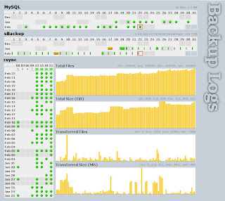
I'm having a bit of trouble figuring out how to describe this. It's a page that shows the current status and history of my backup strategy, and hopefully it's fairly obvious what's going on.

Each time the rsync process runs, the results are logged to a text file. A python routine parses the log file to determine the time the rsync was run, the number of files copied etc.

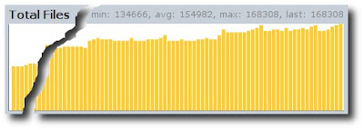
A little calendar indicates if a copy was made in each time slot of the day, this gives an interesting indication of when my computer is switched on. A histogram at the top shows the all time counts, the calendar only shows the last 30 days.

I'm using the Google Chart API to graph the number of files, total size, number of files copied and size of files copied.

The results of sbackup are determined by looking at the dated backup files and their sizes and graphed on a calendar. The size of the incremental and full backups are plotted on separate scales.

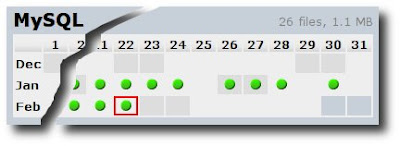
I'm also running a dump from MySQL once a day.

Sunday, February 17, 2008

Podcast and Audiobook Queue Visualisation

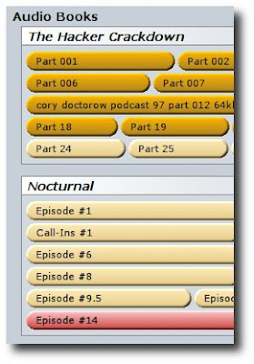
Some screenshots of a little web app I created to visualise my podcast and audio book listening queue:

This shows files currently on my mp3 player. The width of each file represents it's size, the "window width" being 128mb.

Files that will be copied during the next "sync" are indicated with a red dot. Files are copied according to priority, to fill the player and to have only 3 audio book chapters at any time on the player unless there is nothing else to listen to.

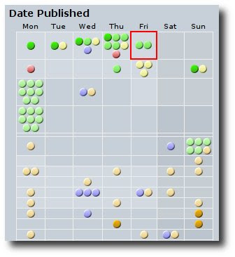
Audio book chapters that have been copied/listened to already are highlighted, as are those that have been downloaded but not yet queued.

The displayed title is taken from the id3 tags if possible, otherwise the filename is used. Dates and redundant "book titles" are removed from the title if possible to maximise the amount displayed, and there is a "hover panel" to display other details.

There's also a pretty calendar to provide a gauge of the age of podcasts in different categories.

Tuesday, January 22, 2008

Photos by Day of Year

One last "heat-map", by day of the year:

Jan Feb Mar Apr May Jun Jul Aug Sep Oct Nov DecTotal
1174 390 1 21 3 9 13 51 13 10 16 72773
27 332 20 3 13 19 8 19 49 83 20 15588
337 271 13 9 35 7 93 43 115 39 48 40750
46 86 12 19 4 24 30 186 133 38 144 34716
570 99 2 12 4 5 45 49 70 12 74 52494
673 88   5 57 55 29 93 84 166 120 17787
7169 102 2 55 11 83 30 23 123 39 34 49720
8203 206 3 70   20 58 22 88 39 45 20774
9130 88 7 21 4 89 47 15 51 106 12 78648
1065 154 9 17 5 51 51 25 12 146 12 27574
1130 381 6 46 2 100 58 42 42 134 48 1890
1223 199 20 38 13 35 90 38 29 102 48 3638
1336 190 19 23 3 21 115 59 15 49 2 19551
1450 263 23 10 39 7 104 159 70 17 53 23818
1557 197 3 9 14   32 263 21 92 24  712
1637 199 16 39 10 57 10 188 101 60 45 42804
1766 238 23 20 12 22 80 63 69 16 15 2626
18109 223 15 43 12 70 96 54 53 12 5 9701
19163 239 87 117 17 20 20 110 101 14 108 131009
20164 31 52 97 68 31 64 18 105 5 18 37690
21200   32 73 19 21 28 72 37 22 5 10519
22194 16 1 43 1 63 24 21 112 36 7 20538
23287 7 33 80 9 27 80 18 60 5 32 104742
24176 108 3 4 8 16 47 106 49 17 8 187729
25308 31 15 95 28 34 94 159 56 5 46 3331204
26239 4 15 4 23 50 46 70 88 41 3 90673
27307 24 3 43 15 32 7 67 65 51 41 71726
28239 11 4 43 10 6 26 14 49 41 10 13466
29166   20 7 11 11 32 3 6 24 32 11323
30278   4 36 22 10 27   54 77 44 104656
31336   7   13   17 83   32   192680
Total4399 4177 470 1102 485 995 1501 2133 1920 1530 1119 168821519

Interesting that there are still some "holes" in there after 8 or so years.

Photos by Time of Day

Another "heat-map", photos by time of day for each day of the week:

12am 1 2 3 4 5 6 7 8 9 10 11 12pm 1 2 3 4 5 6 7 8 9 10 11Total
Mon                                                                                                2449
Tue                                                                                                2828
Wed                                                                                                2774
Thu                                                                                                2658
Fri                                                                                                2545
Sat                                                                                                4395
Sun                                                                                                3870
Total222138341281826328360617122319121938182620492094198419781248962137655038922721519

(Hover for a tooltip indicating the actual number of photos in each 15 minute segment.)